6 Vector Geometries

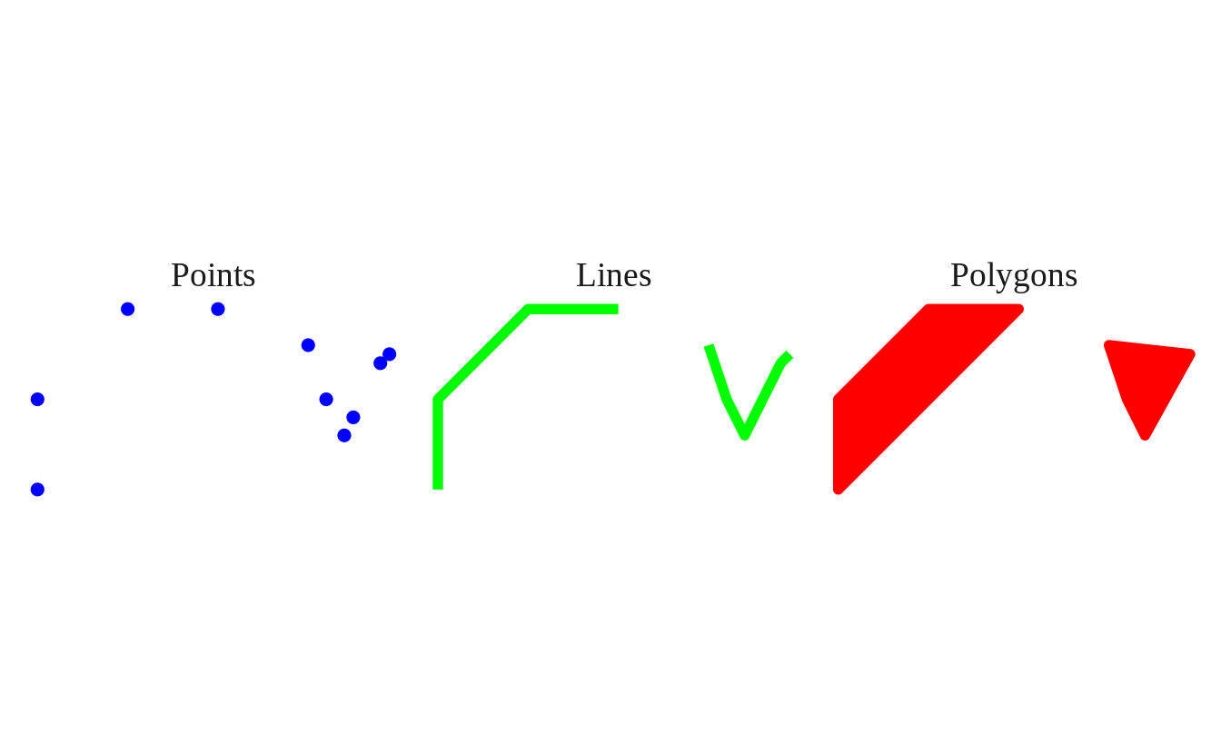
Spatial vector data represent the world as a collection of points which, for two-dimensional data, are stored as \(x\) and \(y\) coordinates.

suppressPackageStartupMessages(library(tidyverse))
library(sf)
#> Linking to GEOS 3.7.1, GDAL 2.4.2, PROJ 5.2.0

theme_spatial <- theme_minimal(base_family = "serif") +
  theme(axis.text = element_blank(), axis.title = element_blank(),
        axis.ticks = element_blank(), panel.grid = element_blank(),
        plot.title = element_text(hjust = 0.5))

theme_set(theme_spatial)

Points can be joined in order to make lines, which themselves can be joined to make polygons.

practice_coords <- tibble(
  lng = c(-20, -20, -10, -10, 20, 20,  10,  10), 
  lat = c(-20, 10, 20, -10, -10,  10,  20, -20),
  lab = c("A", "B", "C", "D", "E", "F", "G", "H"),
  grp = c("a", "a", "a", "a", "b", "b", "b", "b")
)

practice_coords
#> # A tibble: 8 x 4
#>     lng   lat lab   grp  
#>   <dbl> <dbl> <chr> <chr>
#> 1   -20   -20 A     a    
#> 2   -20    10 B     a    
#> 3   -10    20 C     a    
#> 4   -10   -10 D     a    
#> 5    20   -10 E     b    
#> 6    20    10 F     b    
#> 7    10    20 G     b    
#> 8    10   -20 H     b

6.1 `POINT`

POINT refers to the location of a single point in space.

Here, we use st_as_sf() to convert a regular data.frame into an sf object.

Steps:
1. take practice_coords
2. convert to sf object with st_as_sf(), providing a character vector indicating the names of practice_coords in \((x, y)\) / \((longitude, latitude)\) order
3. mutate() to a add a column named shape, which we obtain using st_geometry_type().

point_sf <- practice_coords %>%                     # Step 1.
  st_as_sf(coords = c(x = "lng", y ="lat")) %>%     # 2.
  mutate(shape = st_geometry_type(geometry))        # 3.

point_sf
#> Simple feature collection with 8 features and 3 fields
#> geometry type:  POINT
#> dimension:      XY
#> bbox:           xmin: -20 ymin: -20 xmax: 20 ymax: 20
#> CRS:            NA
#> # A tibble: 8 x 4
#>   lab   grp    geometry shape
#> * <chr> <chr>   <POINT> <fct>
#> 1 A     a     (-20 -20) POINT
#> 2 B     a      (-20 10) POINT
#> 3 C     a      (-10 20) POINT
#> 4 D     a     (-10 -10) POINT
#> 5 E     b      (20 -10) POINT
#> 6 F     b       (20 10) POINT
#> 7 G     b       (10 20) POINT
#> 8 H     b      (10 -20) POINT

The data in our lng and lat columns are moved to a new geometry column.

ggplot(data = point_sf) + 
  geom_sf(aes(color = lab), size = 5, show.legend = "point") +
  labs(title = "POINT")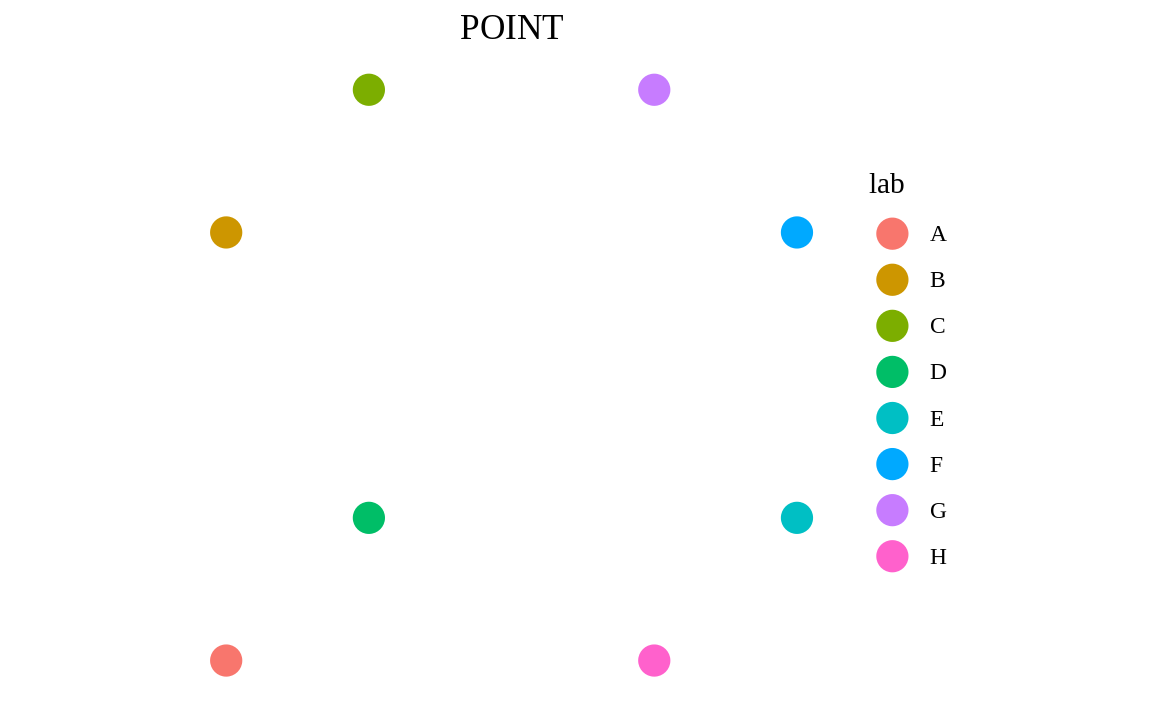

6.2 `MULTIPOINT`

MULTIPOINT refers to a collection of POINTs.

Steps:
1. take point_sf
2. using group_by(), group the rows together based on the values in their grp column
3. summarise() each group, which combines the points of each group into a MULTIPOINT
4. mutate() the shape column to change it to the new st_geometry_type()

multi_point_sf <- point_sf %>%               # Step 1.
  group_by(grp) %>%                          # 2.
  summarise() %>%                            # 3.
  mutate(shape = st_geometry_type(geometry)) # 4.
#> `summarise()` ungrouping output (override with `.groups` argument)

multi_point_sf
#> Simple feature collection with 2 features and 2 fields
#> geometry type:  MULTIPOINT
#> dimension:      XY
#> bbox:           xmin: -20 ymin: -20 xmax: 20 ymax: 20
#> CRS:            NA
#> # A tibble: 2 x 3
#>   grp                                     geometry shape     
#> * <chr>                               <MULTIPOINT> <fct>     
#> 1 a     ((-20 -20), (-20 10), (-10 -10), (-10 20)) MULTIPOINT
#> 2 b         ((10 -20), (10 20), (20 -10), (20 10)) MULTIPOINT

Instead of the 8 separate POINTs with which we started, we now have 2 rows of MULTIPOINTs, each of which contain 4 points.

ggplot(data = multi_point_sf) + 
  geom_sf(aes(color = grp), size = 5, show.legend = "point") +
  labs(title = "MULTIPOINT")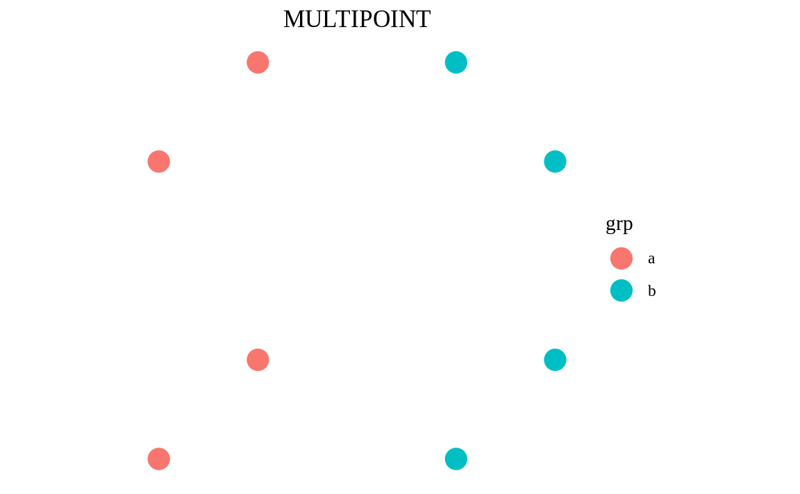

6.3 `LINESTRING`

LINESTRING is how we represent individual lines.

Steps:
1. take multi_point_sf
2. cast the geometry to= LINESTRING using st_cast() 3 mutate() the shape column to change it to the new st_geometry_type()

linestring_sf <- multi_point_sf %>%          # Step 1.
  st_cast(to = "LINESTRING") %>%             # 2.
  mutate(shape = st_geometry_type(geometry)) # 3.

linestring_sf
#> Simple feature collection with 2 features and 2 fields
#> geometry type:  LINESTRING
#> dimension:      XY
#> bbox:           xmin: -20 ymin: -20 xmax: 20 ymax: 20
#> CRS:            NA
#> # A tibble: 2 x 3
#>   grp   shape                                geometry
#> * <chr> <fct>                            <LINESTRING>
#> 1 a     LINESTRING (-20 -20, -20 10, -10 -10, -10 20)
#> 2 b     LINESTRING     (10 -20, 10 20, 20 -10, 20 10)

Now we have 2 rows that each contain a LINESTRING, which was built by connecting each point to the next.

ggplot(data = linestring_sf) + 
  geom_sf(aes(color = grp), size = 2, show.legend = "line") +
  labs(title = "LINESTRING")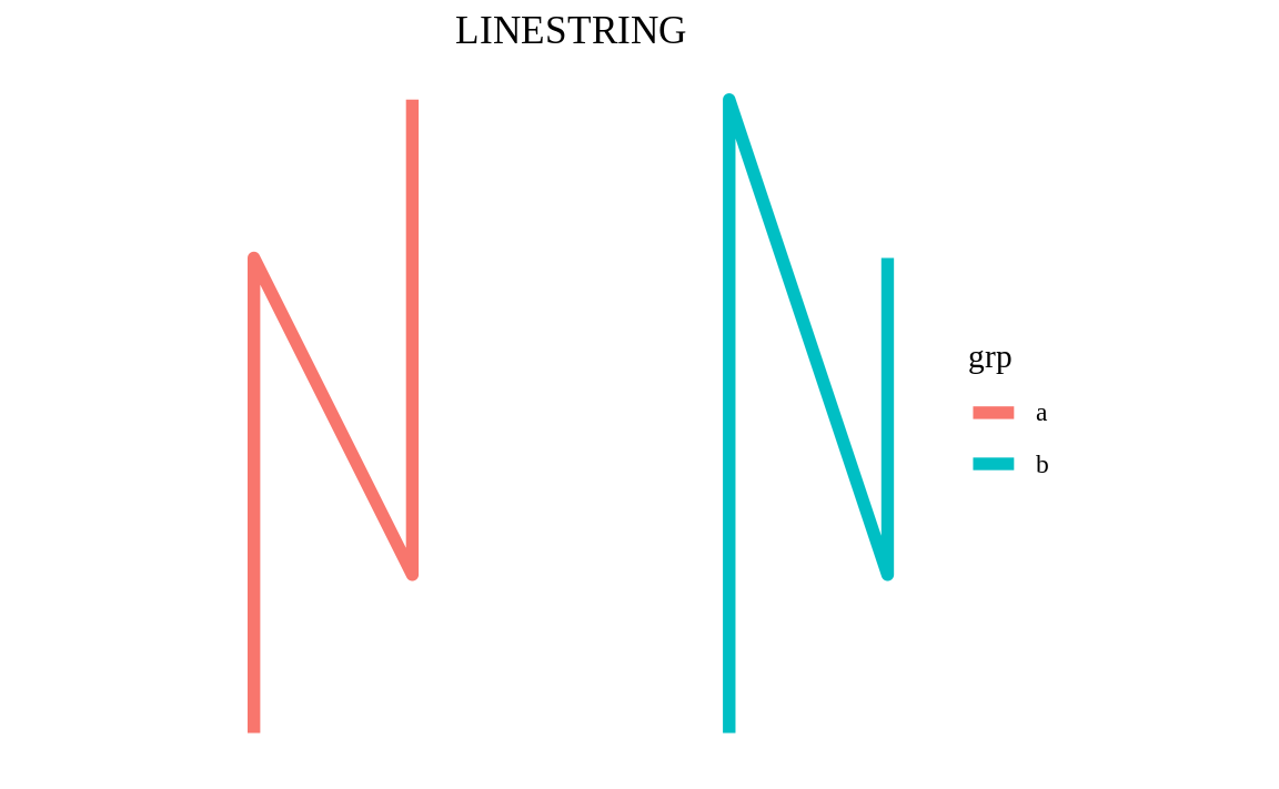

6.4 `MULTILINESTRING`

Similar to MULTIPOINTs that contain multiple points, we also have MULTILINESTRINGs.

Steps:
1. take linestring_sf
2. summarise() the rows, combining them all into a single MULTILINESTRING
3. mutate() the shape column to change it to the new st_geometry_type() and replace the grp column that is dropped when we summarise() without using group_by()

multi_linestring_sf <- linestring_sf %>%     # Step 1.
  summarise() %>%                            # 2.
  mutate(shape = st_geometry_type(geometry), # 3.
         grp = "multi")                      # 4.

multi_linestring_sf
#> Simple feature collection with 1 feature and 2 fields
#> geometry type:  MULTILINESTRING
#> dimension:      XY
#> bbox:           xmin: -20 ymin: -20 xmax: 20 ymax: 20
#> CRS:            NA
#> # A tibble: 1 x 3
#>                                                               geometry shape           grp  
#> *                                                    <MULTILINESTRING> <fct>           <chr>
#> 1 ((-20 -20, -20 10, -10 -10, -10 20), (10 -20, 10 20, 20 -10, 20 10)) MULTILINESTRING multi

Now we have 2 lines embedded inside a single MULTILINESTRING row.

ggplot(data = multi_linestring_sf) + 
  geom_sf(aes(color = grp), size = 2, show.legend = "line") +
  labs(title = "MULTILINESTRING")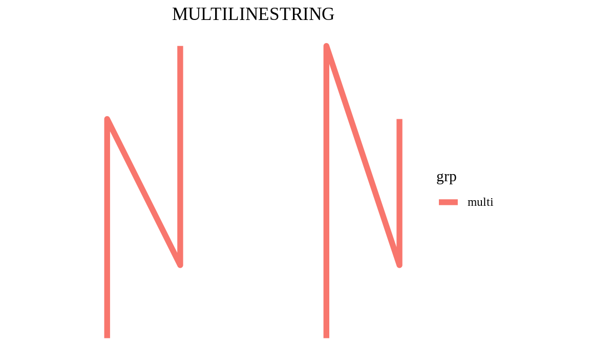

6.5 `POLYGON`

POLYGONs are essentially sets of lines that close to form a ring, although POLGYONs can also contain holes. We can easily wrap a shape around any geometry using st_convex_hull() to form a convex hull polygon.

Steps:
1. take point_sf
2. using group_by(), group the rows together based on the values in their grp column
3. summarise() each group, combining them into MULTIPOINTs
4. wrap the MULTIPOINTs in a polygon using st_convex_hull()
5. mutate() the shape column to change it to the new st_geometry_type()

polygon_sf <- point_sf %>%                   # Step 1.
  group_by(grp) %>%                          # 2.
  summarise() %>%                            # 3.
  st_convex_hull() %>%                       # 4.
  mutate(shape = st_geometry_type(geometry)) # 5.
#> `summarise()` ungrouping output (override with `.groups` argument)

polygon_sf
#> Simple feature collection with 2 features and 2 fields
#> geometry type:  POLYGON
#> dimension:      XY
#> bbox:           xmin: -20 ymin: -20 xmax: 20 ymax: 20
#> CRS:            NA
#> # A tibble: 2 x 3
#>   grp                                        geometry shape  
#> * <chr>                                     <POLYGON> <fct>  
#> 1 a     ((-20 -20, -20 10, -10 20, -10 -10, -20 -20)) POLYGON
#> 2 b          ((10 -20, 10 20, 20 10, 20 -10, 10 -20)) POLYGON

ggplot(data = polygon_sf) + 
  geom_sf(aes(fill = grp), show.legend = "polygon") +
  labs(title = "POLYGON")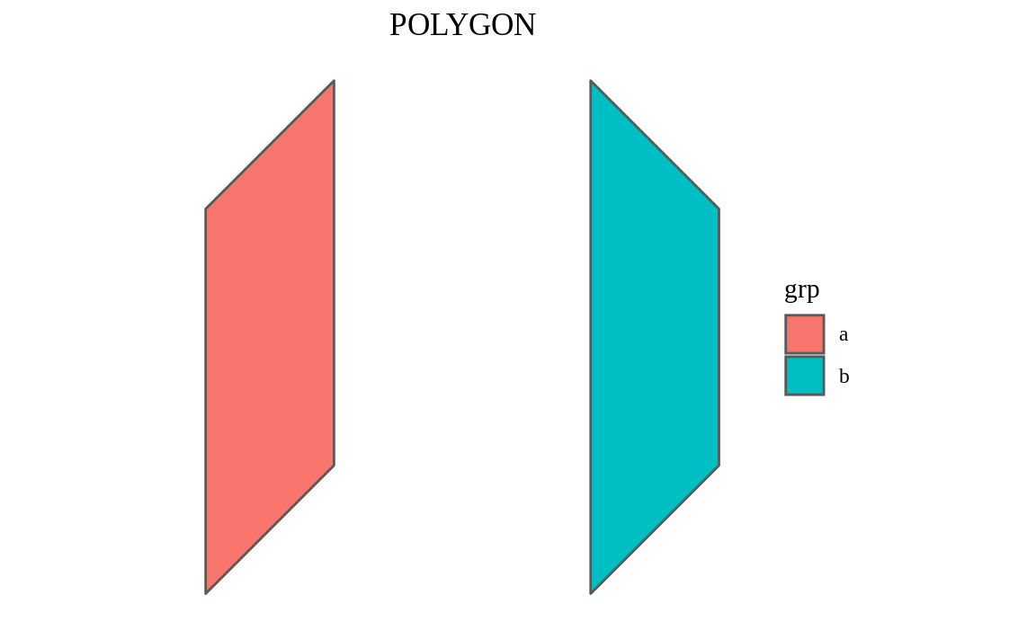

6.6 `MULTIPOLYGON`

POLYGONs can also be grouped together to form MULTIPOLYGONs.

Steps:
1. take polygon_sf
2. summarise() the rows, combining them all into a single MULTILIPOLYGON
3. mutate() the shape column to change it to the new st_geometry_type() and replace the grp column that is dropped when we summarise() without using group_by()

multi_polygon_sf <- polygon_sf %>%           # Step 1.
  summarise() %>%                            # 2.
  mutate(shape = st_geometry_type(geometry), # 3.
         grp = "multi")

multi_polygon_sf
#> Simple feature collection with 1 feature and 2 fields
#> geometry type:  MULTIPOLYGON
#> dimension:      XY
#> bbox:           xmin: -20 ymin: -20 xmax: 20 ymax: 20
#> CRS:            NA
#> # A tibble: 1 x 3
#>                                                                       geometry shape      grp  
#> *                                                               <MULTIPOLYGON> <fct>      <chr>
#> 1 (((-20 -20, -20 10, -10 20, -10 -10, -20 -20)), ((10 -20, 10 20, 20 10, 20 … MULTIPOLY… multi

ggplot(data = multi_polygon_sf) +
  geom_sf(aes(fill = grp), show.legend = "polygon") +
  labs(title = "MULTIPOLYGON")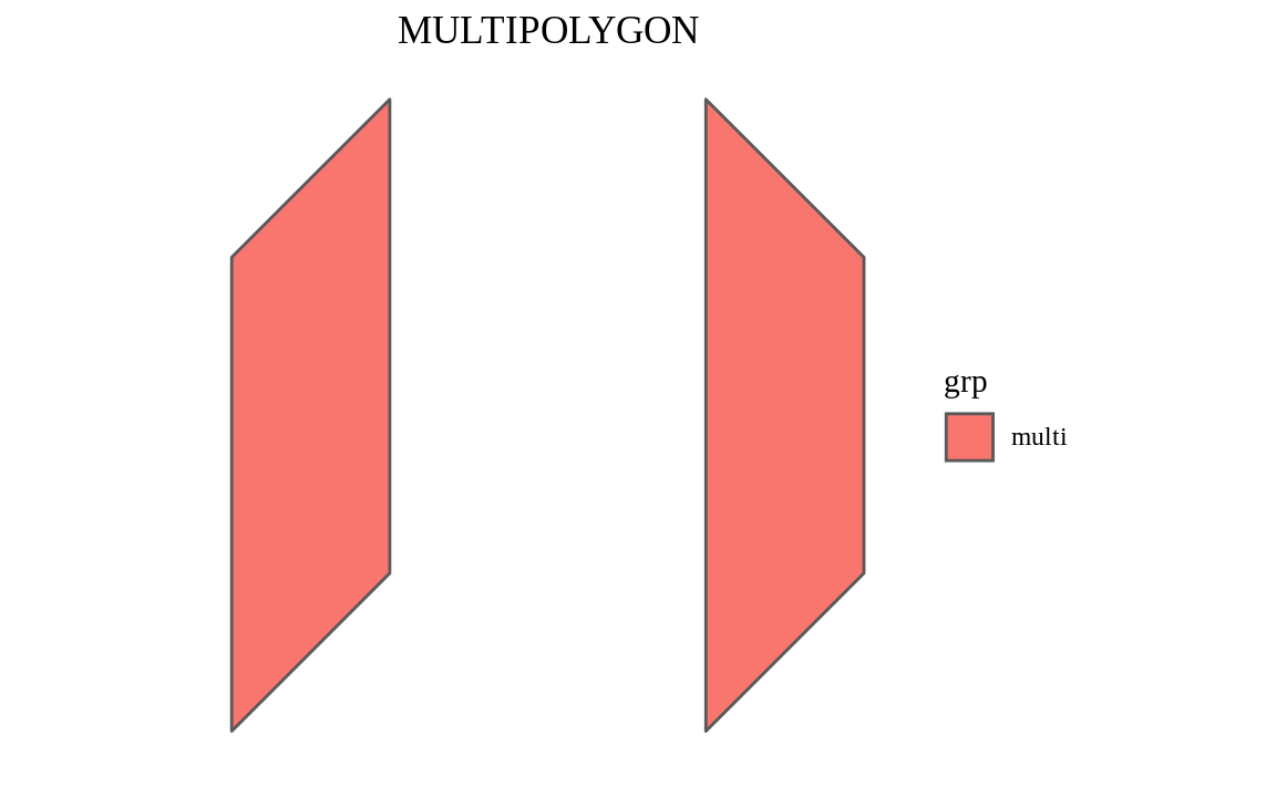

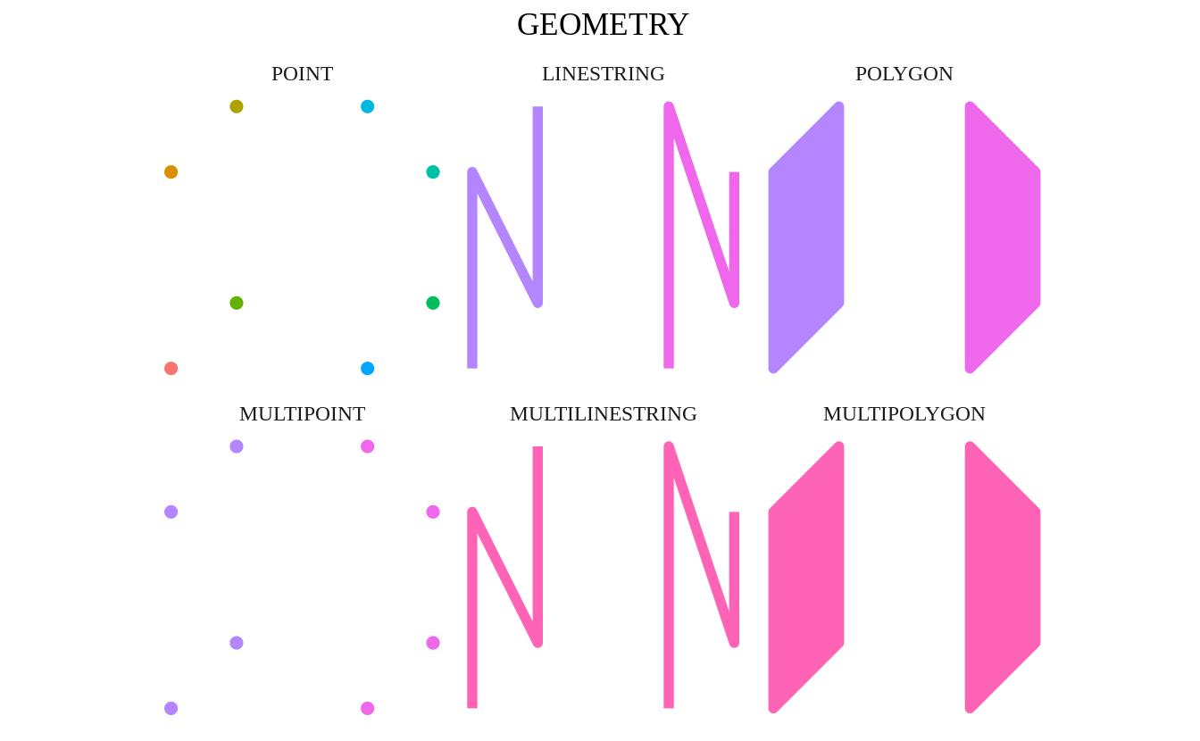
6.7 `GEOMETRY`

GEOMETRY is a special geometry type. It refers to a column of mixed geometries, i.e. we have multiple geometry types in our geometry column.

geometry_sf <- list(point_sf, multi_point_sf, linestring_sf, 
                    multi_linestring_sf, polygon_sf, multi_polygon_sf) %>% 
  map_if(~ "lab" %in% names(.x), select, -lab) %>%
  do.call(what = rbind) %>% 
  mutate(grp = if_else(shape == "POINT", as.character(row_number()), grp))

geometry_sf
#> Simple feature collection with 16 features and 2 fields
#> geometry type:  GEOMETRY
#> dimension:      XY
#> bbox:           xmin: -20 ymin: -20 xmax: 20 ymax: 20
#> CRS:            NA
#> # A tibble: 16 x 3
#>    grp                                                                    geometry shape       
#>  * <chr>                                                                <GEOMETRY> <fct>       
#>  1 1                                                               POINT (-20 -20) POINT       
#>  2 2                                                                POINT (-20 10) POINT       
#>  3 3                                                                POINT (-10 20) POINT       
#>  4 4                                                               POINT (-10 -10) POINT       
#>  5 5                                                                POINT (20 -10) POINT       
#>  6 6                                                                 POINT (20 10) POINT       
#>  7 7                                                                 POINT (10 20) POINT       
#>  8 8                                                                POINT (10 -20) POINT       
#>  9 a                         MULTIPOINT ((-20 -20), (-20 10), (-10 -10), (-10 20)) MULTIPOINT  
#> 10 b                             MULTIPOINT ((10 -20), (10 20), (20 -10), (20 10)) MULTIPOINT  
#> 11 a                                 LINESTRING (-20 -20, -20 10, -10 -10, -10 20) LINESTRING  
#> 12 b                                     LINESTRING (10 -20, 10 20, 20 -10, 20 10) LINESTRING  
#> 13 multi MULTILINESTRING ((-20 -20, -20 10, -10 -10, -10 20), (10 -20, 10 20, 20 … MULTILINEST…
#> 14 a                         POLYGON ((-20 -20, -20 10, -10 20, -10 -10, -20 -20)) POLYGON     
#> 15 b                              POLYGON ((10 -20, 10 20, 20 10, 20 -10, 10 -20)) POLYGON     
#> 16 multi MULTIPOLYGON (((-20 -20, -20 10, -10 20, -10 -10, -20 -20)), ((10 -20, 1… MULTIPOLYGON

ggplot(data = geometry_sf) +
  geom_sf(aes(color = grp, fill = grp), size = 2, show.legend = FALSE) +
  facet_wrap(~ shape, nrow = 2) +
  labs(title = "GEOMETRY")

6 Vector Geometries

6.1 POINT

6.2 MULTIPOINT

6.3 LINESTRING

6.4 MULTILINESTRING

6.5 POLYGON

6.6 MULTIPOLYGON

6.7 GEOMETRY